Graphs
1. Introduction
In this chapter, we will talk about graphs. A graph is a way to represent pieces of data and the connections between them. Visually, they somewhat resemble binary trees, but without limits on the number of children a node can have and without any sort of obvious root.
Here is a basic, graph with 7 vertices (or nodes) and 12 edges (connections between two nodes):
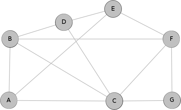
A graph is a collection of vertices (nodes) and edges (connecting the nodes). This is frequently written as G = <V, E>
Vertices are nodes in a graph that can be connected by edges.
An edge in a graph is a connection between two vertices.
Edges can be directed or undirected, and can even have a weight. (More on weight later.)
A path is a sequence of vertices connected by edges.
The degree of a vertex is the number of edges incident to it. (Incident, in this case, means the number of edges leaving a vertex.)
1.1. A Practical Example
Imagine that I am building an apartment and I need to figure out the best way to run the electrical wiring between the rooms. Here is a copy of my floorplan:
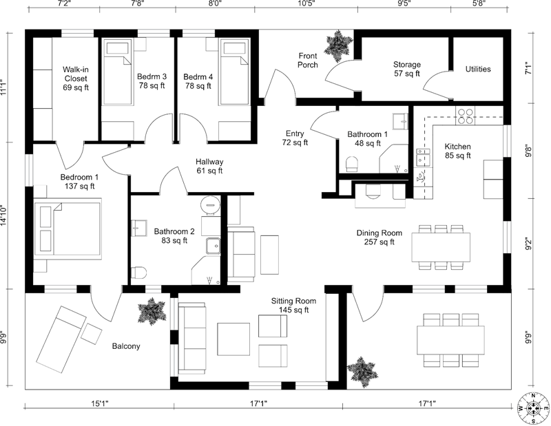
When running my electrical wiring, there are only certain places it can go. For example, I could run wires directly between Bedroom 3 and Bedroom 4 through the wall, but I could not directly connect Bedroom 3 to the Dining Room because that would require running the wire through the middle of the apartment, which would look bad.
To model this, I make a graph showing which rooms (the vertices) could be connected for wiring purposes:

This is a graph representation of how my rooms could be connected by electrical wires. For example, the Hall could be wired directly to Bedroom 3, Bedroom 4, Bedroom 1, or Bathroom 2. The Hall can’t be wired directly to Bathroom 1. This can be seen quickly on the graph.
1.2. Weighted vs. Unweighted Graphs
An unweighted graph is one where the only information implied by an edge is that two vertices are connected. Here, again, is our original graph from the introduction:
The existence of the edge from A to B simply means that there is a direct connection between A and B.
A weighted graph is one where the edges also include a weight which is used to communicate something about the cost associated with that edge. Here is the same graph as before, but now with weights on the edges:
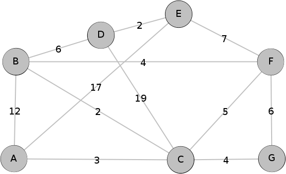
Now, the edge from A to B has a weight of 12. Exactly what this weight means will vary depending on what data is being represented. Note that the length of the edge is not related to its weight.
1.3. Weighted vs. Unweighted Graphs in Our Example
Let’s return to our apartment example. We already have a basic, unweighted graph showing how wires could be run:
Let’s modify that graph to also represent how much wire (in meters) would be required to connect two rooms. (The connection distance between some rooms may be further than others.)

Now the graph tells us that if we want to run wire from the Balcony to the Sitting Room, we will need 5 meters of it.
2. Minimum Spanning Tree
Once you have a graph representing something, there are various algorithms you can run on that graph to learn useful things or solve problems related to the graph. Let’s return to our apartment example. I have a graph that shows me how much wire it would take to connect rooms. Running every possible wire would be expensive, time-consuming, and unnecessary. What is the minimum amount of wire I can use and still manage to make sure every room is connected to electricity?
A minimum spanning tree (MST) is the graph that contains the least total edge weight while still ensuring every vertex is connected to the graph. Here is an MST for our apartment:
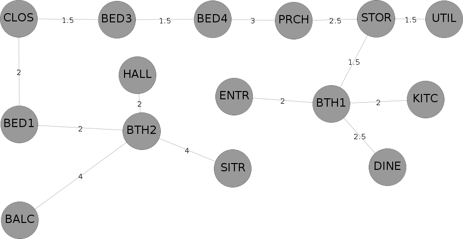
This graph shows us that we can connect all the rooms using only 32 meters of wire. You’ll notice that many edges have been removed because they are not needed.
So, if you are given a graph, how do you determine the minimum spanning tree? Let’s discuss two different algorithms.
The descriptions below describe the algorithms but don’t give examples. We will work examples of these in class.
2.1. Kruskal’s Algorithm
Kruskal’s algorithm for finding an MST was published by Joseph Kruskal in 1956.
It works as follows:
Draw the graph without any edges (so just the vertices).
Sort all the edges, by weight, in ascending order.
While there are edges left and we don’t yet have an MST…
- Select the smallest edge
- Check if adding this edge to the graph would create a cycle
- If no cycle, then add the edge to the graph
- Repeat for the next smallest edge
A graph has a cycle if there is a path in the graph that starts and ends on the same vertex. Informally, a cycle is when the edges form a loop.
The efficiency of this algorithm is \(O(E\textrm{ log }E)\), where \(E\) is the number of edges in the graph.
2.2. Prim’s Algorithm
Prim’s algorithm for finding an MST was published by Robert Prim in 1957, one year after Kruskal’s algorithm. However, it was first discovered by Czech mathematician Vojtěch Jarník.
It works as follows:
Draw the graph without any edges (just draw the vertices).
Choosing an arbitrary vertex, add its smallest edge.
While we don’t yet have an MST…
- Add the edge with the shortest distance from vertices in the MST to a vertex that is not yet in the MST.
Depending on how the graph is stored and the data structure used to implement this algorithm, the efficiency is either \(O(V^2)\) or \(O(E\textrm{ log }V)\), where \(E\) is the number of edges in the graph and \(V\) is the number of vertices.
3. Shortest Path with Dijkstra
Another useful operation to perform on a graph is to find the shortest path between two nodes.
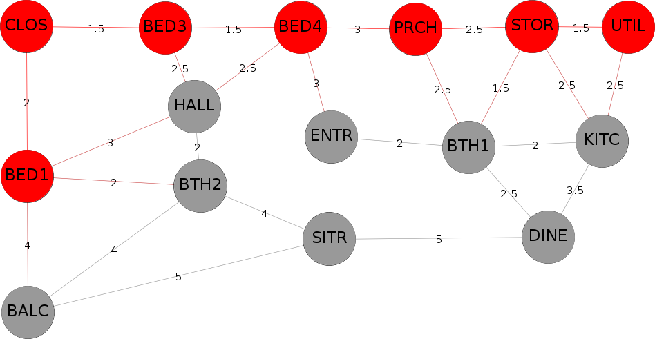
Once again returning to our apartment example, imagine that after I move in I realize that I want to run a network cable from the utility room (where my internet connection enters the house) to bedroom 1, where I keep my home office. I want to find the shortest path to run the cable. Here it is, marked in red:
A common algorithm used for the shortest path problem was developed by Dutch physicist Edsger Dijkstra (who did a lot of work on algorithms) in 1959. The story goes that he developed it over tea with his fiance.
The algorithm does a bit more than find the shortest path between two nodes. It finds the shortest path between a source node and every other node in the graph.
We will work an example using Dijkstra’s algorithm in class. If you would like to see another example, here is a nice one that can be found online.
4. Credits
The floor plan picture is courtesy of Room Sketcher and can be found here